2 years ago
Remember the anxiety felt back in the 1990s after the publications of the first quantum algorithms by Deutsh and Jozsa (1992), Shor (1994), and Grover (1996). Most of us expected quantum computers to be of practical use within a decade, at most two, and numerous popular publications depicted the soon-to-arrive bright era of unlimited computing power under everyone's desk. Three decades later, we still have only prof-of-concepts, claims-to-fame, and bulky contraptions. And sporadic articles of another “important step forwards” along a seemingly endless road. What was, and still is the biggest promise, turns out to be the biggest nightmare as well; exponential speed-up, also means exponentially growing operators to be precisely designed and controlled, and exponentially growing noise to be battled against. Perhaps one day all these obstacles will be removed, but until then it's an ongoing lesson in patience.
Meanwhile, another revolution is quietly sprouting without much of a hype, because thankfully the media is busy foaming elsewhere. Independently, from two directions, scientists and engineers are converging on the idea of moving from digitally processed probabilities to probabilistically processed digits. Spikes are the Mother Nature's choice for macroscopic quanta of information, and we are left to ponder why is this the case.
Into the world of spikes
Spikes may have accidentally appeared in some cells that later specialized into neural tissue facilitated by the information transmission properties of the invention. But one can also argue the opposite, that early neurons may have communicated via electrochemical potentials only with their direct neighbors, and that axons, dendrites, and eventually spikes evolved gradually as communication means along increasing distances. There are still such cells present in the sensory tissues which pre-date brains.
Spikes are quite different from the kind of processing used in electronics, where the two binary states of 0 and 1 are symmetric in terms of stability. Rather than the states themselves, spikes may represent the derivatives of transitions between them.
From a technical point of view, the appearance of spikes might have come from their ability to carry out information even if traveling long distances across a body, in the same way that digital signals can be correctly decoded despite attenuation over the cables. Propagating analogue signals is not feasible in the long run due to the exponential spreading of probability distributions. In contrast, spikes are like decisions, each marking a new stepping stone to support oneself on and dart further from. A good example here are the language models: at each step of text generation one token is selected based on the estimated probability over the vocabulary. If we tried to avoid these decisions, instead of an indicator, a whole probability distribution would be propagated to the next step as an initial condition. After a few steps like this, the distribution would become so uniform, that it would carry no meaning at all. This is fairly similar to forecasting the weather, a system which is so chaotic that predicting it more than several days ahead is bound to fail.
Our digital revolution is based on the same premise: that discrete signals are far more durable than analogue ones. The difference lies in the encoding of states and communication protocols.
For a long time scientist have been trying to decode the language of spikes. Some of the neuromorphic hardware (NMHW) that was built since then are purely for the purposes of simulating the brain. To many of those working in the field of machine learning this sounds like resource squandering, because simulating one system with another is typically some orders of magnitude more expensive. So, they build their own neuromorphic chips, but instead of simulating, the aim is to probe the advantages of alien talk reduced to the bare minimum.
Power efficiency
In the overheating world where never-satiated users demand ever more power-consuming gadgets, the only way forward is to significantly boost the efficiency of the devices. So rather unsurprisingly, the most mundane reason to replace ANNs running on GPUs, with spiking neural networks (SNNs) on NMHWs, is their low energy consumption. Just as graphic processors outperformed CPUs in terms of computational efficiency, so are NMHWs destined to take over neural inference from GPUs:
- First, the major difference between GPU and CPU is that the former comprises multitude of far simpler and less capable "little CPUs", whose sheer number and orchestrated parallelism more than compensate for their individual weakness. Likewise, NMHW divides the work into even smaller processing units—the neurons—each with just one simple algorithm to execute around the clock.
- Second, the processing bottleneck of the von Neumann architecture is the memory access. Modern chips improve on the original idea by adding successive levels of caches (L1, L2, L3...), which significantly reduce transfers. Basically, the more local a computation, the more efficient it is. Neurons, whether biological or electronic, draw information only from their connected neighbors, and this makes them very local. And because all connections are stored on the chip, it's a bit like using exclusively the L1-level cache.
- Third, spikes are events, and a network of spiking neurons is event-driven. This means that only the necessary information is sent through the wires at a time. By contrast, the networks implemented on GPUs are like trains running on a schedule: no matter whether packed with passengers or empty, they keep running, with most of the power being consumed on moving the massive carriages around.
Any electronic device that cannot enjoy the comfort of mains electricity and needs a battery, is a potential beneficiary of neuromorphic HW. The range of such utilities is broad, including for example:
- medical wearables that are used for vital function monitoring.
- military or rescue equipment, such as drones, navigation, sensory enhancement.
- precision agriculture and environmental monitoring which require field sensors in remote areas.
- dormant systems designed for low-rate event detection.
Reducing power consumption by an order of magnitude can prolong battery life several times, which in turn may result in reduced environmental pollution, increased range, or durability of equipment. These are no mean feats, and can sometimes even save lives.
But the applications of NMHW are not limited to power-constrained systems. For example, SpinNNcloud is going to use them in data centers. Indeed, for a computing farm that consumes mega-watts, any improvement in efficiency translates to millions in savings. Something that is well-worth taking into consideration.
The human brain is estimated to consume 12 to 20 watts, even during intense intellectual effort, while an average gaming GPU gobbles an order of magnitude more. Any comparison of their computation capability is loaded with significant uncertainty and a grain of arbitrariness: CPUs, GPUs, and TPUs are typically gauged in FLOPs; for concreteness let’s take FLOP-32, the 32 bit IEEE floating-point operations. On the other hand, the efficiency of NMHWs are estimated in SOPs, the synaptic operations. The relation between the two units varies by orders of magnitude depending on whether we want to simulate spikes in a GPU, or floating-point arithmetic with spikes. Probably the most sensible translation is by comparison of performance on specific tasks and algorithms, for example: a) NorthPole claims 25x better efficiency measured in terms of image frames per joule than Nvidia's V100 GPU on the same task; b) SpiNNaker-2 is over 18x more efficient than A100 GPU; and c) Loihi-2 appears 24x more efficient than Jetson Orin Nano running NsNet2. Given such numbers we can estimate the number of SOPs per FLOPs to be somewhere between 2 and 45 depending on who and how does the counting. On the graph below we assume the ratio to be ~10, and every blue point should be smeared vertically by more than an order of magnitude.
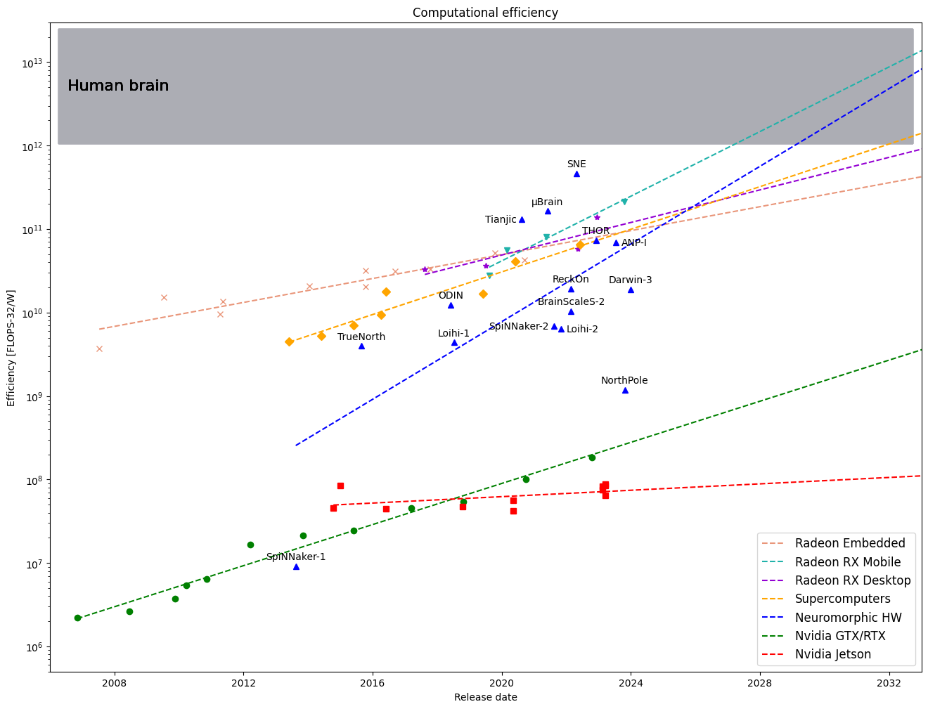
Looking at the mature commercial platforms, AMD Radeon leads the pack. Its mobile RX line, which took over from the discontinued Embedded family, is near the top of efficiency scoreboard. They are on a straight path to enter the human brain efficiency (HBE) zone in about 5 years. Perhaps somewhat unexpectedly, as they consume tens to hundreds of kilowatts, among the best performers are the biggest systems too. Their HBE prediction is about a decade from now.
Towards the bottom of the graph, we find the shining star of capital markets, whose monopolist position seems to nourish complacency rather than competitive edge. Its GTX/RTX gaming line shows no signs of being under pressure; if the trend continues, we will use HBE Nvidia graphics cards sometime in the 2060s. And the Jetson family is heading nowhere in particular, definitely not into the future of IoT, as advertised. The company is green only by its paint, and focused more on holding its grip on the key AI software, than improving its devices.
Finally, neuromorphic hardware is still very diverse and immature, but set on a steep course to achieve the objective of HBE. And because of that diversity and growing competition, the target may be reached even before the 2030s. A very promising direction appears to be Josephson junctions, which according to simulations, could reduce the costs by a further six orders of magnitude, therefore surpassing the brain in efficiency by a wide margin. In the table below, we compile a list of the NMHWs that went public in the last decade.
| platform | developer | release | lit. nm | neurons | synapses | on-device training | freq. MHz | efficiency | library | |||
|---|---|---|---|---|---|---|---|---|---|---|---|---|
| count ↑ | type | count ↑ | type | J/SOP ↓ | W/synapse ↓ | |||||||
| SpiNNaker-1 | Manchester | 2013-08-15 | 130 | 1.60·104 | prog. | 1.60·107 | yes | 150 | 1.13·10-8 | 6.25·10-8 | PyNN | |
| TrueNorth | IBM | 2015-08-28 | 28 | 1·106 | exp-LIF | 2.56·108 | CuBa, Delta | no | async | 4.86·10-11 | 2.54·10-10 | CoreLet |
| ODIN | Louvain | 2018-06-01 | 28 | 2.56·102 | LIF | 6.5·104 | STDP | 75 | 8.40·10-12 | 7.34·10-9 | ||
| Loihi-1 | Intel | 2018-07-10 | 14 | 1.28·105 | LIF | 1.28·108 | CuBa, Delta | STDP | async | 2.36·10-11 | 2.34·10-9 | Lava |
| Tianjic | Tsinghua | 2019-08-01 | 28 | 4.00·104 | prog. | 1.00·107 | no | 300 | 7.82·10-13 | 9.50·10-8 | TJSim | |
| µBrain | Eindhoven | 2021-06-01 | 40 | 3.36·102 | 3.7·104 | no | 1.4 | 6.27·10-13 | 1.97·10-9 | |||
| SpiNNaker-2 | SpiNNcloud | 2021-08-15 | 22 | 1.25·105 | prog. | 1.52·108 | yes | 200 | 1.50·10-11 | 4.67·10-10 | Py-spinnaker-2 | |
| Loihi-2 | Intel | 2021-10-30 | 7 | 1·106 | prog. | 1.28·108 | prog. | prog. | async | 1.61·10-11 | Lava | |
| ReckOn | Zurich | 2022-02-20 | 28 | 2.56·102 | 1.32·105 | e-prop | 13 | 5.47·10-12 | 6.06·10-10 | |||
| BrainScaleS-2 | Heidelberg | 2022-02-24 | 65 | 5.12·102 | AdEx-IF | 1.32·105 | CuBa, Delta | STDP | 1.00·10-11 | PyNN, hxTorch | ||
| SNE | Zurich, Bologna | 2022-04-29 | 22 | 8.19·103 | LIF | no | 400 | 2.21·10-13 | SLAYER | |||
| THOR | Eindhoven, Delft | 2022-12-01 | 28 | 2.56·102 | LIF | 6.5·104 | STDP | 400 | 1.40·10-12 | 1.69·10-7 | ||
| ANP-I | Tsinghua, SynSense | 2023-07-17 | 28 | 5.22·102 | LIF | 5.17·105 | CuBa, Delta | S-TP | 40 | 1.50·10-12 | ||
| NorthPole | IBM | 2023-10-23 | 12 | 1·106 | 2.56·108 | no | async | 8.76·10-11 | NorthPole | |||
| Darwin-3 | Zhejiang | 2023-12-29 | 22 | 2.35·106 | prog. | - | prog. | prog. | 333 | 5.47·10-12 | ||
When comparing the above devices, there are several factors worth taking into account:
- First, the more neurons and synapses the better, because that lets you upload advanced neural models to. You can run simple CNNs on smaller chips, but who needs another MNIST digits classification these days?
- Second, the ratio of synapses to neurons is potentially limiting. Many dense layers require mappings between ~1000 neurons, therefore a good ratio is about 3 orders of magnitude, which is—not coincidentally—similar to the brain. Few devices do satisfy this condition.
- Third, there is the flexibility of implementation: Fixed hardware that offers just one type of neuron (mostly LIF), or single training method (STDP) may be good for the purposes of demonstration but, in practice it's like having only one shoe size for everyone. At least several NMHWs offer programming assemblers which allow you to define their neural operations, at least to some extent.
- Last but not least, there is the issue of power efficiency, but unfortunately there are many ways that one can measure this. The joule per synaptic operation (J/SOP), which is the same as watt per synaptic operations per second (W/SOPS), become the de facto standard. In addition to the expense of individual operations, every platform incurs an overall energy cost, therefore it also makes sense to calculate the average energy consumption per neuron, or better still, per synapse. Usually, the bigger a system, and the more connections it offers, the more efficient it is with respect to this measure.
The actual list of NMHWs is much longer, where most are on the front-line of academic research, and don't even have a catchy name. But some, like Intel Loihi-2, IBM NorthPole, and SpiNNaker-2, have evident commercial ambitions, and are designed with scaling capability in mind. It is very likely that in a couple of years we may witness the first SNN applications in IoT, mobile, and the cloud.
Coding schemes
The first hypothesis about the transmission protocol employed by neurons was a rather unsophisticated rate code, where significance, or probability was proportional to the frequency of spiking. Of course this went up to the limit imposed by the refractory period of ~10 ms, or equivalently ~100 Hz. Unfortunately, the simplest does not mean the most efficient, so a number of more realistic coding schemes have been invented since then, for example: sparse temporal code, intensity to latency, inter-spike interval (ISI), time-to-first-spike (TTFS), phase code, burst code, or phasors on complex-valued neurons. All of them lie somewhere between the rate code and a dense temporal code where every bit matters, as in our digital communications. The in-built negligence of neural synapses makes strict codes unlikely candidates. We don’t know whether this faultiness is just an inescapable property of biological circuitry or an inherent part of information processing adapted to noisy environments. The most likely schemes seem those striking balance between efficiency in terms of spikes per transmitted bit, and the length of decoding temporal window. Such codes may even depend on neuron type and species: the gap in reaction times between e.g. birds and big whales is of several orders of magnitude.
Discovering all of the neural codes may take scientist a long time, but meanwhile we can build spiking neural networks, implement algorithms and observe how they transmit information. This is what many researchers already do.
The spherical cow
Back in the 1952 Hodkin & Huxley published a neuron model, which was so good that with some additions and modifications it is still used today. But what is good for simulation is often bad for computing efficiency, and since then researchers and engineers have reduced the model dramatically from an elaborate system of differential equations down to couple of difference ones, resulting in a kind of spherical cow model.
Integrate and Fire (IF) – This is the principal philosophy behind SNNs. It’s the point of contact between the two main ingredients: potentials vit and actions |sit| ∈ {0, 1}. There are more than few variants of the IF theme, but the core idea remains unchanged: a cell sums up the weighted spikes of its afferent neighbors to modify its own potential, then probabilistically emits its own spike, or keeps quiet. A spike is a discharge, so it significantly alters the cell potential. Depending on the model, it does so by a certain quanta (soft reset), down to a resting value (hard reset), or to an even lower value (reset with refractory period).
In order to make the network sub-critical, it is common to use potential decay (leaky IF) with the decay constant |λ| ≤ 1 as a hyper-parameter. The activation function that maps cell potential to action probability can be linear, quadratic, exponential, and so on.
There are variants that go beyond binary outputs, such as for instance graded spikes: these cells can output any positive integer value, so that their nonlinearity is at least a discretization of potentials. To some extent this can be seen as the time-saving form of spike bursts observed in the natural neurons.
Another variant is the Resonate and Fire model: in the original form it integrates only real spikes, but naturally extends to complex ones, allowing to conveniently handle oscillatory signals that often feature in audio processing.
We can consider SNNs as either an instance of ANNs with a specific kind of activation function, or conversely perceive ANNs as short-time averages over SNNs. The later interpretation, however, is consistent with the rate coding scheme and seems prevalent in the literature.
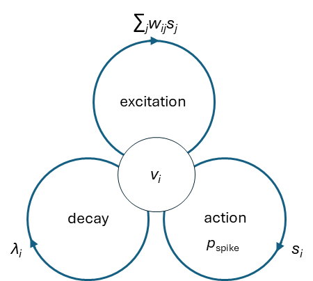
Most of the practical neuron models operate according to the general algorithm:
- Imitate the internal dynamics of true neurons by v → λv, whereas system stability requires |λ| ≤ 1;
- Accumulate weighted signals from afferent neurons into excitatory potential v → v*;
- Probabilistically generate action potential v* → s (spike);
- Relax or reset excitatory potential (v*, s) → v conditioned on emitted spike.
However note that, these are three independent processes affecting the state potential v, which can be executed in arbitrary order, even stochastically, without qualitative change of network functionality:
More formally, it can be put in the following form:
v*it = λi vi(t - 1) + ∑ j wij sj(t - 1), sit = nv*it|v*it|-1 with probability pspike(v*it, n), n = 0,1,2,..., vit = r(v*it, sit),
where pspike is a probability function that estimates the chances of firing n-graded spike given excitatory potential v*it. By default n = 1, pspike(v) = θ(v – vthr) is the Heaviside step function, with a conveniently set threshold vthr = 1. The r is a reset function that reduces the potential after discharge. In hard reset models r(v*, s) = (1 – s)v*, whereas soft reset could mean quantized discharge r(v*, s) = (v* – s). In case of resonant neurons, the state vit, excitation potentials v*it, spikes sit, synaptic weights wij, and decay constant λi, are complex-valued. Note that while the decay rate |λi| is largely neuron-independent, i.e. either constant, or shared among large groups of neurons, the phase ωi := arg(λi) is characteristic of individual neuron. In practice, λi = exp(-1/τm + iωi), where τm ≥ 0 is membrane constant, and ωi ∈ [0, 2π) is neuron's characteristic frequency.
Training with spikes
The first methods to train ANNs were—like the ANNs themselves—inspired by nature. The synaptic weights were trained using Hebb’s rule which famously states that those who fire together, wire together as well. But over the years this method was superseded by much more efficient, although hardly natural backpropagation (BP) of output errors towards the origin. Unlike Hebbian learning, which is local, BP is global, which means that a single adaptation step can modify, albeit minutely, every parameter of the model. Since the first applications back in the 1980s BP has become the dominant training algorithm for all ANN models. Major ANN development frameworks offer no alternative to BP.
SNN researchers quickly realized that they got a problem with their spherical herd. What appeared to be a beautiful simplification turned into a major stumbling block. One of the conditions for BP to be feasible is that the whole transformation is composed of differentiable functions. Point-wise discontinuities of the derivatives can somehow be tolerated as long as they remain defined in the vicinity. That’s the case for instance of the very popular and successful ReLU and MaxPool operations. But in case of SNN the situation is far worse: The default spike generator is a Heaviside step function pspike(v) = θ(re(v) - 1), which not only is not differentiable, it is also discontinuous. This means that the gradient at the firing threshold is a Dirac delta and vanishes elsewhere, which completely ruins the BP.
At first, researchers tried to get back to the Hebbian method, or to bypass the problem and follow the approach of quantized networks converting ANNs to SNNs, but the resulting models were evidently worse than originals.
Those outcomes were hardly encouraging, but thankfully, Mother Nature came to the rescue: in biological computers nothing is exact, neither the potentials vit, nor the firing thresholds vthr. And probably this is for a good reason. Because if we assume that, for instance, due to inherent noise either of the two is normally distributed with standard deviation σ, then the sharp step changes to a familiar sigmoidal function used in ANNs, as illustrated below:
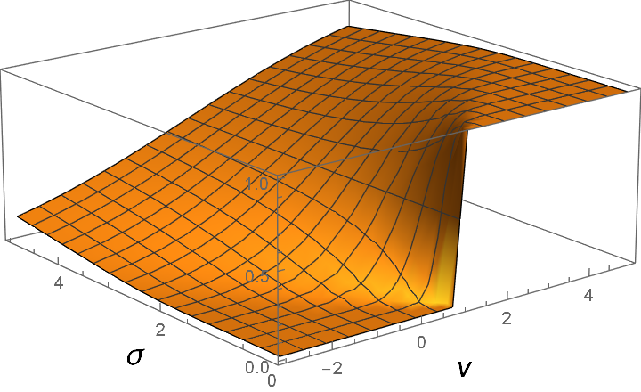
pspike = θ(v - 1) → ½[1 + erf((v – 1)/σ)]
In practice, for the sake of computational simplicity it is common to use arctan for the sigmoid, which corresponds to assuming a Cauchy distribution instead of a Gaussian. Many mathematicians would object to such a maneuver, but from engineering point of view the particular choice doesn't make much of a difference.
Likewise, if our model permits graded spikes, or is running replicas, then the staircase output of the expectation E[n] changes to a soft version of the cherished ReLU activation, which is also differentiable:
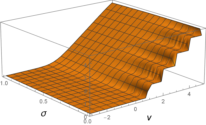
E[n] = ∑ n ≥ 1 θ(v - n) → ½ ∑ n ≥ 1 [1 + erf((v – n)/σ)] ≈ log[1 + exp(e·(v - ½)]/e
This procedure is known as surrogate gradient, and has become the de facto standard in SNN training. However, despite suggestive graphics above, choosing the best surrogate is not a simple matter. That’s because most SNNs still use the sharp step function instead of a smooth probability, so the whole effect depends on the distributions of potentials vit which are a priori unknown.
There are alternative approaches to training SNNs with gradients. We can use, for example, the adjoint state variables derived via Pontryagin’s minimum principle, however they remain computationally rather intensive, and unsurprisingly have not caught on.
Recent advances
Recurrence
The gradient is not the only problem that we face when trying to train SNNs. Since these networks are a special kind of temporal RNNs, it should not be surprising to encounter the vanishing and exploding gradients when using backpropagation through time (BPTT). As a remedy, one of the NMHW platforms is offering eligibility propagation (e-prop) for the on-device training. Another, more biologically plausible approach, though perhaps limited in terms of architecture, is equilibrium propagation (EP), where the network is using two relaxation phases, each with different energy functions to determine the parameter update without explicitly computing the gradient. Perhaps the most viable BPTT alternative is the forward propagation through time (FPTT): By eliminating the costly propagation of gradients through a temporally unrolled network, it achieves a significant reduction in both memory footprint and training time. FPTT means augmenting the loss function with a crafted dynamic regularizer term, and then limiting the gradient to just one step. The authors report experiments with significantly higher accuracies than for reference RNN networks (especially LSTM and GRU) trained with BPTT. The same strategy was successfully applied to spiking networks.
Residual Networks and Transformers
Vanishing gradients means that local minima are separated by long plateaus, that are not feasible to cross. In SNNs, even shallow ones, the issue is particularly pronounced due to aforementioned non-differentiability, which makes even the surrogate gradients very localized. In deep architectures, the remedy was found in the form of residual connections, which directly link distant parts of the network allowing signals to “skip” the heavy sub-modules until they are actually needed. This mechanism was quickly adapted to SNNs, with image classification results similar to those of ANNs. Since then, several teams have reported improvements on this subject.
In temporal domain, instead of residuals, somewhat different approach was found successful: the transformer. By utilizing attention across long time intervals these architectures are able to avoid information decay due to unrolling through time, and hence keep the gradients alive. Two years after residual networks, the spiking self-attention was demonstrated. And this year, a very nice, and fully spike-based approach of stochastic spiking attention was proposed and implemented on FPGA, beating GPU ~20 times in terms of power consumption, and outdoing earlier implementations along the way.
Reversible Blocks
Deep Transformers are beasts so memory-hungry, that training them directly would be prohibitively expensive. In order to perform the back-propagation step it is necessary to keep track of all the network states from input up to output, what can quickly exhaust your memory budget. The idea introduced in the NICE trick was to make the architecture reversible, so that, instead of using memorized states, we could easily re-compute them back when needed. This was one of the breakthroughs that allowed present LLMs to flourish. Soon afterwards, reversible blocks in recurrent architectures were proposed, and recently, such reversible blocks were also implemented with spikes in both Transformers, and RNNs.
The downside
There's a little bit worrying issue that many of these architectures employ operations like batch-norm, which are neither genuinely local and event-driven, nor implementable on the current neuromorphic hardware. Non-local potentials like average and standard deviation present in normalization layers could perhaps be compared to neurotransmitter modulation in the brain, a mechanism that is beyond the ability of our spherical cow. Its absence means that no network using batch-norm, neither the ResNet nor Transformer, could be trained on NMHW.
Another issue, is the inference of probabilities. If anybody hoped for deciphering the neural language by observing communication in artificial spiking networks, spontaneously self-organizing into optimal code, then the current state of the art could be disillusioning. It turns out that vast majority of works use the unimpressive rate code. But who knows, perhaps if left talking to themselves, artificial SNNs may some day discover better ways of exchanging information.
Perspectives
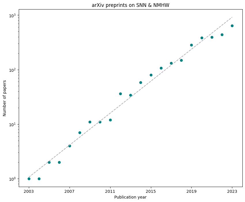
Every new topic in science and engineering starts with a phase of exponential growth in terms of interest. As the arXiv service testifies, that seems to be the case with the spiking neural networks, and neuromorphic hardware, which are on the exponential upward curve in number of publications.
Engineering walks shortly after research, and only in the last year we have seen probably as many applications, as in the previous two decades combined, for example, reinforcement learning, eye-tracking, micro-gesture recognition, audio compression, audio source localisation, voice activity detection, Hebbian learning in lateral circuits, or quadratic programming. If this trend continues, in a year or two NMHW platforms will hit the market an enable low-power SNN AI on mobile mini-devices. And services offering online access to NMHWs not only for development work but also for cloud AI should appear soon afterwards.
Further reading
- Adrian & Zotterman, 1926 “The impulses produced by sensory nerve endings: Part 3. Impulses set up by Touch and Pressure” Journal of Physiology 61, pp. 465–483.
- Bellec et al., 2020 “A Solution to the Learning Dilemma for Recurrent Networks of Spiking Neurons” Nature Communications 11:3625.
- Blouw et al., 2019 “Benchmarking keyword spotting efficiency on neuromorphic hardware” Proceedings of the 7th Annual Neuro-Inspired Computational Elements Workshop, ser. NICE ’19. New York, USA: Association for Computing Machinery.
- Bonazzi et al., 2023 “A Low-Power Neuromorphic Approach for Efficient Eye-Tracking” arXiv:2312.00425.
- Chen et al., 2024 “Noisy Spiking Actor Network for Exploration” arXiv:2403.04162.
- Cheng et al., 2017 “Understanding the Design of IBM Neurosynaptic System and Its Tradeoffs: A User Perspective” DATE '17: Proceedings of the Conference on Design, Automation & Test in Europe, pp. 139–144.
- Davies et al., 2018 “Loihi: A neuromorphic manycore processor with onchip learning” IEEE Micro 38:1, pp. 82–99.
- Deutsh & Jozsa, 1992 “Rapid solution of problems by quantum computation” Procedings of the Royal Society of London A 439, pp. 553-558.
- Diehl et al., 2015 “Fast-classifying, high-accuracy spiking deep networks through weight and threshold balancing” 2015 International Joint Conference on Neural Networks (IJCNN)
- Dinh et al., 2015 “NICE: Non-linear independent components estimation” ICLR 2015.
- Ferris, 2012 “Does Thinking Really Hard Burn More Calories?” Scientific American.
- Frenkel et al., 2019 “A 0.086-mm2 12.7-pJ/SOP 64k-Synapse 256-Neuron Online-Learning Digital Spiking Neuromorphic Processor in 28-nm CMOS” IEEE Transactions on Biomedical Circuits and Systems 13:1 (2019) pp. 145-158.
- Frenkel & Indiveri, 2022 “ReckOn: A 28 nm Sub-mm2 Task-Agnostic Spiking Recurrent Neural Network Processor Enabling On-Chip Learning over Second-Long Timescales” 2022 IEEE International Solid-State Circuits Conference (ISSCC).
- Gautrais & Thorpe, 1998 “Rate coding versus temporal order coding: A theoretical approach” Biosystems 48 pp. 57–65.
- Gomez et al., 2017 “The Reversible Residual Network: Backpropagation Without Storing Activations” 31st Conference on Neural Information Processing Systems (NIPS 2017), Long Beach, CA, USA.
- Grover, 1996 “A fast quantum mechanical algorithm for database search” Proceedings of the 28th annual ACM symposium on Theory of computing - STOC '96. Philadelphia, Pennsylvania, USA: Association for Computing Machinery. pp. 212–219.
- Haghighatshoar & Muir, 2024 “Low-power SNN-based audio source localisation using a Hilbert Transform spike encoding scheme” arXiv:2402.11748.
- Han et al., 2024 “High-speed Low-consumption sEMG-based Transient-state micro-Gesture Recognition by Spiking Neural Network” arXiv:2403.06998.
- Hodkin & Huxley, 1952 “A quantitative description of membrane current and its application to conduction and excitation in nerve” Journal of Physiology 117 (I952), pp. 500-544.
- Höppner et al., 2021 “The SpiNNaker 2 Processing Element Architecture for Hybrid Digital Neuromorphic Computing” arXiv:2103.08392.
- Hu et al., 2020 “Spiking Deep Residual Network” arXiv:1805.01352.
- Izhikevich, 2001 “Resonate-and-fire neurons” Neural Networks 14, pp. 883-894.
- Johansson & Birznieks, 2004 “First spikes in ensembles of human tactile afferents code complex spatial fingertip events” Nature Neuroscience 7, pp. 170–177.
- Kag & Saligrama, 2021 “Training Recurrent Neural Networks via Forward Propagation Through Time” Proceedings of the 38th International Conference on Machine Learning, PMLR 139 (2021), pp. 5189-5200.
- Kayser et al., 2009 “Spike-Phase Coding Boosts and Stabilizes Information Carried by Spatial and Temporal Spike Patterns” Neuron 61:4, pp. 597-608.
- Lisboa & Bellec, 2024 “Spiking Music: Audio Compression with Event Based Auto-encoders” arXiv:2402.01571.
- Ma et al., 2023 “Darwin-3: A large-scale neuromorphic chip with a Novel ISA and On-Chip Learning” arXiv:2312.17582.
- Di Mauro et al., 2022 “SNE: an Energy-Proportional Digital Accelerator for Sparse Event-Based Convolutions” 2022 Design, Automation & Test in Europe Conference & Exhibition (DATE). IEEE, pp. 825–830.
- Mangalore et al., 2024 “Neuromorphic quadratic programming for efficient and scalable model predictive control” arXiv:2401.14885
- Modha et al., 2023 “Neural inference at the frontier of energy, space, and time” Science 382:6668 pp. 329-335.
- Neftci et al., 2019 “Surrogate gradient learning in spiking neural networks: Bringing the power of gradient-based optimization to spiking neural networks” IEEE Signal Processing Magazine 36, pp. 51–63.
- Orchard & Jarvis 2023 “Hyperdimensional Computing with Spiking-Phasor Neurons”"> ICONS'23: Proceedings of the 2023 International Conference on Neuromorphic Systems 22 pp. 1–7.
- Painkras et al., 2013 “SpiNNaker: A 1-W 18-Core System-on-Chip for Massively-Parallel Neural Network Simulation”" IEEE Journal of solid-state circuits 48:8, pp. 1943-1953.
- Pascanu et al., 2013 “On the difficulty of training recurrent neural networks” Proceedings of the 30th International Conference on Machine Learning pp. 1310-1318, Atlanta, Georgia, USA.
- Pehle et al., 2022 “The BrainScaleS-2 accelerated neuromorphic system with hybrid plasticity” Frontiers in Neuroscience 16, 795876.
- Pei et al., 2019 “Towards artificial general intelligence with hybrid Tianjic chip architecture” Nature 572, pp. 106-111
- Plank et al., 2022 “The Case for RISP: A Reduced Instruction Spiking Processor” arXiv:2206.14016.
- Reich et al., 2000 “Interspike Intervals, Receptive Fields, and Information Encoding in Primary Visual Cortex” Journal of Neuroscience 20:5, pp. 1964–1974.
- Rieke et al., 1996 “Spikes. Exploring the Neural Code” The MIT Press.
- Rumelhart et al., 1986 “Learning representations by back-propagating errors” Nature 323:6088 pp. 533–536.
- Sawada et al., 2016 “TrueNorth Ecosystem for Brain-Inspired Computing: Scalable Systems, Software, and Applications” JSC16; Salt Lake City, Utah, USA.
- Scellier & Bengio, 2017 “Equilibrium Propagation: Bridging the Gap between Energy-Based Models and Backpropagation” Frontiers in Computational Neuroscience 11, 24
- Senapati et al., 2022 “THOR - A Neuromorphic Processor with 7.29 GTSOP2/mm2Js Energy-Throughput Efficiency” arXiv:2212.01696.
- Schneider et al., 2018 “Ultralow power artificial synapses using nanotextured magnetic Josephson junctions” Science Advances 4, e1701329.
- Shor, 1994 “Algorithms for Quantum Computation: Discrete Logarithms and Factoring” Proceedings 35th Annual Symposium on Foundations of Computer Science, Santa Fe, NM, USA.
- Shrestha et al., 2023 “Efficient video and audio processing with Loihi 2” arXiv:2310.03251.
- Song et al., 2024 “Stochastic Spiking Attention: Accelerating Attention with Stochastic Computing in Spiking Networks” arXiv:2402.09109.
- Stuijt et al., 2021 “An Event-Driven and Fully Synthesizable Architecture for Spiking Neural Networks” Frontiers in Neuroscience 15, 664208.
- Vaswani et al., 2017 “Attention Is All You Need” 31st Conference on Neural Information Processing Systems (NIPS 2017), Long Beach, CA, USA.
- Werbos, 1990 “Backpropagation through time: what it does and how to do it” Proceedings of the IEEE 78:10, pp. 1550-1560.
- Williams & Zipser, 1989 “A learning algorithm for continually running fully recurrent neural networks” Neural computation 1:2, pp. 270–280.
- Xiao et al., 2024 “Hebbian learning based orthogonal projection for continual learning of spiking neural networks” arXiv:2402.11984.
- Yang et al., 2024 “A robust, low-power, and light-weight voice activity detection with spiking neural networks” arXiv:2403.05772.
- Yin et al., 2021 “Accurate online training of dynamical spiking neural networks through forward propagation through time” arXiv:2112.11231.
- Zeldenrust et al., 2018 “Neural coding with bursts—current state and future perspectives” Frontiers in Computational Neuroscience 12 art. 48.
- Zhang et al., 2023 “ANP-I: A 28 nm 1.5 pJ/SOP asynchronous spiking neural network processor enabling sub-0.1 μJ/sample on-chip learning for edge-AI applications” 2023 IEEE International Solid-State Circuits Conference (ISSCC), pp. 21–23.
- Zhang & Zhang, 2023 “Memory-Efficient Reversible Spiking Neural Networks” arXiv:2312.07922.